Revisiting the problem of heterophily for GNNs

2021-08-03T00:00:00+00:00

Introduction

Fig. 1: Example of a graph with mixed homophily and heterophily, with node colors representing class labels: nodes in green show strong homophily, while nodes in orange and purple show strong heterophily.

Graph neural networks (GNNs) have gained wide research interest for their success in learning with graph data. The limitations of GNNs beyond the commonly assumed homophilous settings (where the connected nodes tend to have the same class labels and similar node features) have been lately attracting significant attention: many works have empirically discovered the degradation of GNN performance on heterophilous datasets and proposed designs aiming at improving the GNN performance under heterophily (where connected nodes may have different class labels and dissimilar features) [1,2,3,4,5,6]; some works have also provided theoretical justifications for the proposed designs [1,3,5,6].

Recently, a preprint by Ma et al. [7] revisited the problem of heterophily for GNNs: they observed that in some synthetic and real-world heterophilous datasets, GCNs [8] could still show competitive performance, in some cases even outperforming models featuring heterophilous designs (such as \(\mathrm{H_2GCN}\) [1]). These observations may seem to be contradictory to the findings of previous works that GCNs do not generally work well on heterophilous graphs. Moreover, the authors questioned whether homophily is always a necessary condition for GCNs to work well, and claimed that “heterophily in and of itself is not a problem for GCNs” [7].

In this post, we explain the reasons behind the seemly contradictory observations between this preprint [7] and our previous work on heterophily [1], and address the questions raised by the authors. We further discuss the differences in the focus and scope of the contributions of [7] and [1], and how the takeaways of both works are compatible with each other. In our discussion below, we assume that the readers are familiar with the claims and analyses of the corresponding works.

Why do the observations of GCN performance on heterophilous graphs seem to be contradictory in [7] and [1]?

The most seemingly contradictory observations between [7] and [1] are probably the takeaways on the synthetic graphs:

[7] shows that on synthetic graphs with few or no randomly-added heterophilous connections (i.e., with the noise parameter \(\gamma\) close to 0 — all the heterophilous edges are added according to the pre-defined compatibility matrix), the performance of GCNs can even increase as the level of heterophily in the graph gets stronger (i.e., when the edge homophily ratio \(h\) decreases),
while the prior work [1] shows that the performance of GCNs significantly decrease with the increase of the level of heterophily.

Our follow-up analysis shows that these seemingly contradictory results are due to the different processes used to generate the synthetic graphs with varying level of homophily in [7] and [1,2]:

[7] generates them by adding a large number of heterophilous (cross-label) edges on top of existing (homophilous) real-world graphs like Cora and Citeseer.
[1,2] follow a modified preferential attachment process which allows to control the edge homophily ratio (or, more generally, the class compatibility matrix) of the resulting graph, while maintaining the power-law degree distribution.

These two synthetic graph generation processes lead to very different properties (e.g., degree distribution, class compatibility matrix) in the resulting graphs, which in turn affect the model performance, as we will discuss in the next section.

Looking deeper into the conditions for GCNs to work well on heterophily

In [7], the authors attribute the key reason of competitive performance of GCNs on heterophilous graphs to the intra-class similarity and inter-class distinguishability of the class label distributions of the 1-hop neighbors for nodes in the graphs: when nodes in the same class have strong similarities in neighborhood label distributions, and nodes from different classes have weak or no similarities, the GCNs are able to perform well due to the high distinguishability of the neighborhood label distributions, even when the graphs are heterophilous.

Our analysis in general agrees with this finding, but we also find that the high distinguishability of the class label distributions under heterophily is largely dependent on the properties of the graphs, such as degree distributions, and underlying compatibility matrices (which is also addressed in [7] in their Observation 2). In the following discussion, to explain how these graph properties can affect the distinguishability of the neighborhood label distributions in heterophilous settings, we use as examples two sets of synthetic graphs generated from cora: (1) denser synthetic graphs used in [7] (which we call necessity-cora) and (2) sparser synthetic graphs based on the generation process in [1,2] (which we refer to as syn-cora).

The effect of low-degree nodes

📌 In Observation 2 in [7], the authors state that

if the neighborhood label distributions of nodes \(v \in \mathcal{V}_c\) are sampled from a fixed distribution \(\mathcal{D}_c\), and
when \(c \neq c'\), the distributions \(\mathcal{D}_{c}\) and \(\mathcal{D}_{c'}\) are distinguishable from each other,

then it is expected that the GCN models can perform well in the heterophilous settings.

However, the aforementioned statement ignores a critical point about the varied quality of the samples of the distribution \(\mathcal{D}_c\) under varied degrees for each node \(v \in \mathcal{V}_c\): when all the nodes have sufficiently large degrees, it is expected that \(\mathcal{D}_c\) can be recovered well in the node neighborhoods due to sufficient samples of the distributions; however, when many low-degree nodes are present in the graph (which is the case for many real-world graphs, which usually follow power-law degree distributions), \(\mathcal{D}_c\) may not be consistently recovered in the neighborhood of the low-degree nodes under heterophily due to the insufficiency of the samples. This affects the intra-class and inter-class similarity of the neighborhood label distributions in heterophilous settings.

Low-degree nodes & Heterophily

We can further explain how low-degree nodes affect the intra-class and inter-class similarity of the neighborhood label distributions for GCNs under heterophily using the following toy examples.

Empirical Setup: Suppose the neighborhood label distributions \(\mathcal{D}_c\) and \(\mathcal{D}_{c'}\) for two classes \(c \neq c'\) are given in the red dashed boxes in Fig. 2; following the distributions \(\mathcal{D}_c\) and \(\mathcal{D}_{c'}\), we randomly generate the neighborhood label distributions of 200 nodes with degree 2 for both classes by sampling the labels of their 2 neighbors independently from the corresponding underlying distribution, and we visualize 10 of the 200 synthetic neighborhood label distributions below (clustered with the corresponding ground-truth distribution in the dashed red box).

We note that as the formulation of GCN aggregators additionally consider a self loop for each node, the neighborhood label distribution observed by GCN models should be considered with self loops added to the graphs, even when \(\mathcal{D}_c\) and \(\mathcal{D}_{c'}\) dictate purely heterophilous connections. To visualize the effects of self loops in the neighborhood label distributions, we visualize their contributions to the distributions in Fig. 2 (and its follow-up figures) in gray.

Fig. 2: (a) Neighborhood label distribution \(\mathcal{D}_c\) of class \(c\), which shows strong heterophily, in the red dashed box, with visualizations of 10 of the 200 synthetic neighborhood label distributions sampled from \(\mathcal{D}_c\) under node degree of 2. (b) Neighborhood label distribution \(\mathcal{D}_{c'}\) of another class \(c'\), which also shows strong heterophily, in the red dashed box, with visualizations of 10 of the 200 synthetic neighborhood label distributions sampled from \(\mathcal{D}_{c'}\) under node degree of 2. For both plots, the gray parts visualize the contributions of self loops in the neighborhood label distributions aggregated by GCN.

Observations: (1) From Fig. 2, we observe that the intra-class neighborhood label distributions have a high variance and can be very different from the corresponding ground-truth distributions (even when not considering the self loops). In fact, the mean and standard deviation of the intra-class pairwise cosine similarity among the 200 synthetic neighborhoods of class \(c\) and \(c'\) are \(0.79\pm 0.24\), where the high standard deviation reflects the strong variance among the sampled neighborhood distributions.

(2) Furthermore, we observe that many of the neighborhood label distributions from nodes in class \(c, c'\) are the same when considering the self loops, which affects the distinguishability of the neighborhood label distributions between different classes; the inter-class pairwise cosine similarity for our synthetic neighborhoods of class \(c\) and \(c'\) is \(0.79\pm0.17\) in this case, which is the same as the intra-class pairwise similarity with even smaller standard deviation.

High-degree nodes & Heterophily

On the other hand, when the node degrees are high under heterophily, the neighborhood label distributions are more similar to the underlying distributions \(\mathcal{D}_c\) and \(\mathcal{D}_{c'}\) (even with self loops considered) and thus have much smaller variances. In Fig. 3, we illustrate randomly sampled neighborhood label distributions of another 200 nodes with degree 10 (instead of 2). The mean and standard deviation of the pairwise cosine similarity among the generated neighborhoods of class \(c\) and \(c'\) are \(0.93\pm0.09\), while the inter-class pairwise similarity decreased to \(0.64\pm0.15\). These changes in intra-class and inter-class similarities can also be observed from the illustrations of the sampled distributions below.

Fig. 3: (a) Neighborhood label distribution \(\mathcal{D}_c\) of the same class \(c\) as in Fig. 2, with visualizations of 10 of the 200 synthetic neighborhood label distributions sampled from \(\mathcal{D}_c\) under node degree of 10. (b) Neighborhood label distribution \(\mathcal{D}_{c'}\) of the same class \(c'\) as in Fig. 2, with visualizations of 10 of the 200 synthetic neighborhood label distributions sampled from \(\mathcal{D}_{c'}\) under node degree of 10. For both plots, the gray parts visualize the contributions of self loops in the neighborhood label distributions aggregated by GCN.

Connection to prior work

From the above analysis, we see that the existence of low-degree nodes can lead to weak distinguishability of inter-class neighborhood label distributions, thus affecting the performance of GCNs. Our empirical analysis in previous works has supported this observation, where we observed significant performance gap between low-degree and high-degree nodes for H2GCN under heterophily [1]; we show the results of this corresponding empirical analysis in [1] on the right.

Furthermore, we believe that the Observation 2 in [7], which aligns with their empirical observations, have missed the lack of low-degree nodes as a necessary condition for good GCN performance under heterophily due to the approach of introducing heterophily to the necessity-cora synthetic graphs: the necessity-cora graphs with homophily ratio \(h<0.5\) (i.e., heterophilous) have a much higher average degree compared to their corresponding base graph cora, as large amount of edges need to be added in order to decrease the edge homophily ratio in the (strongly homophilous) base graph.

As an example, in Fig. 4, we show the degree distribution of base graph cora in comparison to the degree distributions of the necessity-cora graphs with \(\gamma=0\) (i.e., when all the heterophilous edges are added according to the pre-defined compatibility matrix, without any randomness) under various edge homophily ratios \(h\). We see that as \(h\) decreases, the degrees for all nodes in the graph grow, and the degree distributions move further away from the degree distribution of cora; for the \(h=0.077\) instance, even the minimum node degree in the necessity-cora graph has exceeded the degree of most nodes in cora. In our further empirical analysis, we show that the lack of low-degree nodes is indeed a necessary condition that contributes to the observed high performance of GCNs on necessity-cora.

Fig. 4: (a) Zipf plot of degree distribution of cora, which shows a typical power-law degree distribution. (b) Zipf plot of the degree distribution of necessity-cora, the cora-based synthetic graphs in [7] with \(\gamma=0\) and edge homophily ratio \(h\in \{0.077, 0.303, 0.446, 0.584, 0.789\}\). As \(h\) decreases, the degrees for all the nodes increase, and the degree distributions are moving further away from the original degree distribution of cora.

Degree & Homophily

An important note to add to the above discussion is that the presence of low-degree nodes does not affect the similarity of neighborhood label distributions as much in strong homophilous settings as in the heterophilous settings. In the example below, we similarly generate the neighborhood label distributions of 200 nodes with degrees of 2 for class \(c, c'\), but this time with distributions \(\mathcal{D}_c\) and \(\mathcal{D}_{c'}\) showing strong homophily. From Fig. 5 below, we observe that, unlike the heterophilous settings, almost all synthetic distributions of nodes from the same class \(c\) (or \(c'\)) are close to the expected distribution \(\mathcal{D}_c\) (or \(\mathcal{D}_{c'}\)); most neighbors (considering self-loops) have the same class label \(c\) (or \(c'\)) as themselves, even for low-degree nodes. The intra-class pairwise cosine similarity among the synthetic neighborhoods of class \(c\) and \(c'\) in these homophilous settings is \(0.88\pm0.15\) and \(0.91\pm0.13\), respectively. On the other hand, the inter-class pairwise similarity is \(0.21\pm0.29\), which shows good separability. This example shows that the presence of low-degree nodes is a challenge that is more pronounced in heterophilous settings than in homophilous settings.

Fig. 5: (a) Neighborhood label distribution \(\mathcal{D}_c\) of class \(c\), which now shows strong homophily, in the red dashed box, with visualizations of 10 of the 200 synthetic neighborhood label distributions sampled from \(\mathcal{D}_c\) under node degree of 2. (b) Neighborhood label distribution \(\mathcal{D}_{c'}\) of another class \(c'\), which also shows strong homophily now, in the red dashed box, with visualizations of 10 of the 200 synthetic neighborhood label distributions sampled from \(\mathcal{D}_{c'}\) under node degree of 2. For both plots, the gray parts visualize the contributions of self loops in the neighborhood label distributions aggregated by GCN.

The effect of compatibility matrices

Another factor that affects the distinguishability of inter-class neighborhood label distributions is the distinguishability of the prescribed \(\mathcal{D}_c\) for different classes: when the node degrees are sufficiently high, the neighborhood node distributions for nodes \(v \in \mathcal{V}_c\) are expected to follow \(\mathcal{D}_c\), as we discussed in the previous section; in this case, as stated in Observation 2 in [7], the distinguishability of inter-class neighborhood label distributions mostly depends on the distinguishability of \(\mathcal{D}_c\). Using the terminology in [1,2], the distribution \(\mathcal{D}_c\) for each class \(c\) can be modeled by the compatibility matrix \(\mathbf{H}\), where each row represents the expected neighborhood label distribution \(\mathcal{D}_c\) of the corresponding class \(c\); when the rows of \(\mathbf{H}\) are distinct, the condition of the Observation 2 in [7] holds with sufficiently high node degrees, and it is expected that the GCN models will perform well.

Heterophily

The differences in the distinguishability of the compatibility matrices \(\mathbf{H}\) can also explain the differences in the observed performance of GCN on necessity-cora and syn-cora. In the top row of Fig. 6, we visualize the compatibility matrices of graphs from necessity-cora and syn-cora with homophily ratio \(h\) around 0.0 (i.e., pure heterophily):

when \(\gamma=0\), the compatibility matrices in necessity-cora are formulated to resemble a \(k\)-partite graph, where almost all connections of class \(c\) are limited to the two adjacent classes;
in comparison, the heterophilous connections of class \(c\) in syn-cora are distributed to all classes \(c'\neq c\), and the rows of the compatibility matrix are less distinct.

From the cosine similarity of the compatibility matrices (the bottom row of Fig. 6, i.e., cosine similarity between \(\mathcal{D}_c\) and \(\mathcal{D}_{c'}\) for pairwise classes \(c\) and \(c'\)), we can also see that

the \(k\)-partite heterophilous connection patterns introduced by necessity-cora when \(\gamma=0\) help maintain the high distinguishability of \(\mathcal{D}_c\) among different classes, and thus provide an easier node classification problem for GCNs compared to more general heterophilous patterns;
in comparison, the high similarity of \(\mathcal{D}_c\) among different classes in syn-cora makes it hard to distinguish different classes from the neighborhood label distributions even for high degree nodes, as many heterophilous connections from class \(c\) are uniformly distributed to other classes \(c'\neq c\), similar to the \(\gamma=0.8\) setup of necessity-cora.

Fig. 6: (Top row) Comparison of compatibility matrices of different synthetic graphs. (Bottom row) Comparison of the cosine similarity of the rows in the compatibility matrices (i.e., cosine similarity between \(\mathcal{D}_c\) and \(\mathcal{D}_{c'}\) for pairwise classes \(c\) and \(c'\)) of different synthetic graphs.

Homophily

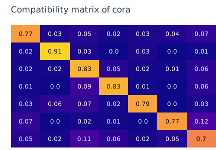
We also note that as similarly discussed in the Observation 1 in [7], the distinguishability of \(\mathcal{D}_c\) (or the distinctiveness of the rows in compatibility matrix \(\mathbf{H}\)) is guaranteed for graphs with strong homophily, as the largest weights in the distributions are concentrated along the diagonal elements of the compatibility matrix \(\mathbf{H}\) for homophilous graphs; as an example, we show the compatibility matrix of cora in the plot. Thus, the distinguishability of the neighborhood label distributions \(\mathcal{D}_c\) is also a challenge specific to heterophilous settings.

Further Empirical Analysis

We conduct additional empirical studies to evaluate the above analysis regarding the effects of low-degree nodes and compatibility matrices (specifically, \(k\)-partite connections) to GCN performance on heterophilous graphs.

To study the effects of these two factors in a more fine-grained way, we generate an additional set of synthetic graphs which have \(k\)-partite heterophilous connections similar to necessity-cora (by leveraging the same or similar compatibility matrices as specified in [7] in the generation process), but the same power-law degree distribution as syn-cora (by following the same modified preferential attachment generation process as in [1,2]). We refer to this new set of synthetic graphs as necessity-cora-ours, and consider two variants:

necessity-cora-ours-5: with 5 classes based on syn-cora and
necessity-cora-ours-7: with 7 classes based on necessity-cora.

In Fig. 7, We additionally visualize the degree distributions and compatibility matrices of necessity-cora-ours-5 and necessity-cora-ours-7, along with the visualizations for necessity-cora and syn-cora:

Fig. 7: Degree distributions (left column) and compatibility matrices (right column) of the graphs evaluated in our empirical studies.

Performance of different models on synthetic graphs

We compare the performance of H2GCN, GCN and MLP on the four sets of synthetic graphs to examine how the degree distributions and compatibility matrices affect the performance of these GNN models; for necessity-cora and syn-cora, we select the graph with \(h\) closest to 0 (i.e., closest to the \(h=0\) target as specified in [7]). For each model, we report the average and standard deviation of the classification accuracy of each model under 5 runs with different random seeds per dataset.

Setup. For GCN, we follow the same hyperparameter tuning as in [7], and additionally tune the dimension of hidden embeddings between 16 and 64. For H2GCN, we tune only a subset of the hyperparameters that we tune for GCN (16 vs. 112 combinations, which are more hyperparameter combinations than those explored in [1]). We use the provided training, validation and test splits for necessity-cora, and generate the splits in similar ways for necessity-cora-ours and syn-cora. In the following table, we list the performance of each model along with the corresponding properties of the graphs:

Name	# Nodes	# Edges	Edge Homo. Ratio \(h\)	H2GCN-2 Accuracy (%)	H2GCN-1 Accuracy (%)	GCN Accuracy (%)	MLP Accuracy (%)
necessity-cora [7] (\(\gamma=0\))	2708	132196	0.03	\(99.26\pm0.28\)	\(93.48\pm0.93\)	\(100.00\pm 0.00\)	\(59.16\pm0.52\)
necessity-cora-ours-7	2708	5394	0	\(88.45\pm1.26\)	\(80.85\pm1.69\)	\(65.10\pm1.80\)	\(58.20\pm2.05\)
necessity-cora-ours-5	1490	2968	0	\(87.98\pm1.49\)	\(82.40\pm 1.77\)	\(59.26\pm2.17\)	\(64.16\pm1.61\)
syn-cora [1]	1490	2968	0	\(68.95\pm1.88\)	\(66.82\pm2.13\)	\(27.27\pm1.72\)	\(63.84 \pm2.17\)

Results. In the table above, we can see the effects of low-degree nodes and \(k\)-partite connections to the performance of GNN models when the graphs share similar edge homophily ratio \(h\):

With no low-degree nodes and \(k\)-partite heterophilous connections, models like GCN and H2GCN-2 can achieve near-perfect accuracy on necessity-cora.
When we keep the \(k\)-partite patterns in the compatibility matrices but modify the degree distributions to follow a power law, we observe 34.90% to 40.74% decrease in accuracy for GCN, which falls below the accuracy of H2GCN on these graphs (though the performance of H2GCN also decreases in this case).
If we further strip the \(k\)-partite connectivity patterns for heterophilous connections, on syn-cora, the performance of GCN further decreases by 31.99% and falls much below the performance of the graph-agnostic MLP in this case; though the accuracy of H2GCN variants also decreases significantly, they still outperform MLP in this case.

The significant changes in the accuracy of GCN can also be explained by the changes in the neighborhood label similarity as discussed in [7]: here, we similarly calculate the neighborhood label similarity for the all synthetic graphs following Eq. (8) in [7], except that we do not take into account the similarity of each node with itself into the average (i.e., when \(c = c'\) and \(i=j\) in Eq. (8) in [7]). In addition, we also calculate the standard deviation of the similarity. Below in Fig. 8, we visualize the calculated cross-class neighborhood similarity and observe the following:

With the presence of low-degree nodes, the necessity-cora-ours variants have lower similarity and higher variance for intra-class neighborhood label distributions compared to necessity-cora, though they share similar compatibility matrices and \(k\)-partite connection patterns;
The removal of the \(k\)-partite patterns in the compatibility matrices of syn-cora further reduces the similarity for intra-class neighborhood label distributions, and increases the inter-class similarity of neighborhood label distributions, leading to weak distinguishability of the neighborhood label distributions between nodes from different classes.

These observations explain the decrease of GCN performance observed in our experiments, and show how that the distinguishability of the neighborhood label distributions can depend on other properties like degree distributions and compatibility matrices in the graphs.

Fig. 8: Cross-class neighborhood similarities of the graphs evaluated in our empirical studies.

Is heterophily still a problem for GCNs? Do we still need designs for heterophilous graphs?

As GCNs are able to achieve competitive performance on some synthetic and real-world heterophilous graphs under certain conditions (i.e., when the distinguishability of the neighborhood label distributions is high), a natural follow-up question is whether heterophily is still a problem worth studying for GNNs. Our view is: yes, heterophily is still a challenging problem for GNN models, including GCN.

From the above discussions, we have revealed that in order to achieve high separability of neighborhood label distributions under heterophily, the graph needs to satisfy certain properties, including having few low-degree nodes (which may not comply with the power-law degree distribution) and having distinct rows in the class compatibility matrix (e.g., \(k\)-partite heterophilous connections). However, these conditions are not always realized in real-world graphs, and in these cases GCNs are still not able to perform well, as the authors show from the synthetic graph experiments with higher values of \(\gamma\) (or noise in the cross-class connections) in [7]. Thus, we believe that it is also an important research question to propose designs to improve the performance of GNNs under more generally conditioned heterophilous settings.

Furthermore, as we have discussed in the previous sections, the factors which hinder the distinguishability in neighborhood node distributions are uniquely challenging under heterophilous settings: in strong homophilous settings (e.g., Cora and Citeseer), the compatibility matrix \(\mathbf{H}\) has by default distinct rows, and low-degree nodes also have smaller effect to the separability of neighborhood node distributions. That also explains why previous works on strong homophilous graphs do not look into the issue of distinguishability in neighborhood label distributions nor the factors that affects the distinguishability.

GCN vs. H2GCN

Next, we show that the GNN designs for heterophilous settings that we identified in [1] can largely improve the performance of GNNs compared to GCNs when the heterophilous connections do not have the ideal distinguishability in the neighborhood label distributions as in the \(\gamma=0.0\) case. Following the experiment setup in the previous set of experiments, we run GCN, two variants of H2GCN and MLP on a subset of the necessity-cora synthetic dataset generated in [7]. We visualize the performance of the four models in Fig. 9. We observe that:

when more heterophilous connections follow the random pattern instead of the prescribed \(k\)-partite pattern (i.e., when \(\gamma\) is high), H2GCN variants largely outperforms GCN under heterophilous settings;
when \(\gamma\) is low (more heterophilous edges following the prescribed \(k\)-partite pattern), we also observe that H2GCN outperforms GCN under higher homophily ratio \(h\) (i.e., with less \(k\)-partite heterophilous edges added and more low-degree nodes), which confirms our above-mentioned analysis.

📌 In summary,

the heterophilous designs we identified in [1] aim at utilizing effectively the heterophilous graph adjacency information under general conditions, with focus on preventing the performance of GNNs from degrading more than the performance of MLP;
on the other hand, [7] focuses more on exploring the GCN performance for heterophilous graphs under specific conditions.

Fig. 9: Performance of H2GCN variants, GCN and MLP on necessity-cora under various \(\gamma\) and edge homophily ratio \(h\). This figure is interactive: hover the mouse on data points to see the exact values; click the legends on the right to toggle the visibility of each model.

Our Takeaways

[7] brings into light how the performance of GCNs can vary based on the distinguishability of the neighborhood label distributions in heterophilous graphs; such analysis is missing in the previous works addressing heterophily, and the competitive performance of GCNs on certain synthetic and real-world heterophilous datasets also clarified the fact that homophily is not always a necessary assumption for GCNs to work well. However, in our follow-up analysis, we have also shown that the high separability of the neighborhood label distributions is dependent on specific graph properties like degree distribution and compatibility matrix under heterophily. Moreover, we showed that such dependence is an especially critical challenge in heterophily settings since it has much weaker effects under homophily settings. Therefore, we believe that the heterophily-specific limitations and challenges for GNN models are still there: the work of [7] and our previous works [1,2] have provided some complementary perspectives of how the performance of GNNs can be affected by the heterophilous settings; how to design a GNN model that effectively combines the advantages of GCN on idealized conditions (with high node degrees and separable compatibility matrices) and H2GCN on more general heterophilous conditions remains an open research question.

Acknowledgements

We thank Yao Ma for sharing with us the synthetic datasets generated for the experiments in Section 3.2 of [7], Yujun Yan for the thoughtful discussions in preparing this post, and Yao Ma, Xiaorui Liu, Neil Shah and Jiliang Tang for the constructive discussions regarding the takeaways of this post.

References

[1]Jiong Zhu, Yujun Yan, Lingxiao Zhao, Mark Heimann, Leman Akoglu, and Danai Koutra. 2020. Beyond Homophily in Graph Neural Networks: Current Limitations and Effective Designs. Advances in Neural Information Processing Systems 33, (2020).
[2]Jiong Zhu, Ryan A Rossi, Anup Rao, Tung Mai, Nedim Lipka, Nesreen K Ahmed, and Danai Koutra. 2021. Graph Neural Networks with Heterophily. In Proceedings of the AAAI Conference on Artificial Intelligence, 11168–11176.
[3]Sami Abu-El-Haija, Bryan Perozzi, Amol Kapoor, Nazanin Alipourfard, Kristina Lerman, Hrayr Harutyunyan, Greg Ver Steeg, and Aram Galstyan. 2019. Mixhop: Higher-order graph convolutional architectures via sparsified neighborhood mixing. In international conference on machine learning, PMLR, 21–29.
[4]Hongbin Pei, Bingzhe Wei, Kevin Chen-Chuan Chang, Yu Lei, and Bo Yang. 2019. Geom-GCN: Geometric Graph Convolutional Networks. In International Conference on Learning Representations.
[5]Deyu Bo, Xiao Wang, Chuan Shi, and Huawei Shen. 2021. Beyond Low-frequency Information in Graph Convolutional Networks. In Proceedings of the AAAI Conference on Artificial Intelligence, 3950–3957.
[6]Yujun Yan, Milad Hashemi, Kevin Swersky, Yaoqing Yang, and Danai Koutra. 2021. Two Sides of the Same Coin: Heterophily and Oversmoothing in Graph Convolutional Neural Networks. arXiv preprint arXiv:2102.06462 (2021).
[7]Yao Ma, Xiaorui Liu, Neil Shah, and Jiliang Tang. 2021. Is Homophily a Necessity for Graph Neural Networks? arXiv preprint arXiv:2106.06134 (2021).
[8]Thomas N. Kipf and Max Welling. 2017. Semi-Supervised Classification with Graph Convolutional Networks. In International Conference on Learning Representations (ICLR).

Jiong Zhu